X 射线与 XMM-Newton EPIC

X-rays and XMM-Newton EPIC

X 射线是能量在 \(0.1\) 到 \(10\ \mathrm{keV}\) 左右的光子（本项目主要用 \(0.4\) 到 \(12\ \mathrm{keV}\)）。它看不见、穿不过大气，所以必须用卫星。XMM-Newton 是欧空局 1999 年发射的 X 射线望远镜，至今仍在运行。

X-rays are photons with energies of roughly \(0.1\) to \(10\ \mathrm{keV}\) (this project mainly uses \(0.4\) to \(12\ \mathrm{keV}\)). They are invisible and cannot pass through the atmosphere, so they need a satellite. XMM-Newton is an ESA X-ray telescope launched in 1999 and still operating.

它有三台相机。本项目只用其中两台：MOS1 与 MOS2（合称 MOS，Metal-Oxide-Semiconductor 相机，每台由 7 块 CCD 环形排成）。第三台 pn 更快但背景更难减，只做交叉检查。为什么 MOS 优先？因为 pn 的 QPB 归一化依赖视场角区，而那里有光子漏进来，导致 pn 的 QPB 被高估——这是本项目已量化的一个缺陷。

It carries three cameras. This project uses two of them: MOS1 and MOS2 (together MOS, Metal-Oxide-Semiconductor cameras, each made of 7 CCDs arranged in a ring). The third, pn, is faster but its background is harder to subtract, so it is a cross-check only. Why MOS first? Because the pn QPB is normalised from the field corners, where photons leak in, so the pn QPB is over-estimated — a defect this project has quantified.

每次观测有一个标识号 ObsID（例如 0763120101）。一次观测指向天空一个方向，曝光几万秒。同一块天可以被不同的 ObsID 在不同时间、以不同离轴角看到——这正是本项目利用的杠杆。

Each observation has an identifier, the ObsID (for example 0763120101). One observation points at one direction of the sky for tens of thousands of seconds. The same piece of sky can be seen by different ObsIDs at different times and at different off-axis angles — that is exactly the lever this project uses.

来源：Source: MosaicSelfCal/problems/v4/r240/M31/problems.csv

两种背景：QPB 与 SP

Two backgrounds: the QPB and soft protons

探测器自己会数出很多"光子"，它们不是从天空来的。有两种，性质完全不同：

The detector itself counts many "photons" that do not come from the sky. There are two kinds, with completely different characters:

• 准静态粒子背景（QPB，quiescent particle background）。宇宙线、大气中微子、地球反照等高能粒子穿过探测器，激发出与 X 射线无法区分的信号。它"安静"——随时间大致稳定，能量谱硬（高能端比例大），在空间上大致均匀。ESAS 的做法是：把视场角区（探测器上看不到天空的那部分 CCD）的计数按面积比例放大，当作整个孔径的 QPB。 The quiescent particle background (QPB). Cosmic rays, atmospheric neutrinos and Earth-albedo particles pass through the detector and produce signals indistinguishable from X-rays. It is "quiescent" — roughly constant in time, hard in spectrum (a large fraction at high energy), and roughly uniform in space. ESAS estimates it by taking the counts in the field corners (the CCD area that sees no sky) and scaling them by area.
• 软质子（SP，soft protons）。太阳风里的低能质子被地球磁场暂时捕获、聚焦到探测器上，能量低（软），在时间和空间上都剧烈变化：一阵一阵来，视场中心和边缘强度不同。它没有"安静时段"可以借用，只能用一段时间模板去减。 Soft protons (SP). Low-energy protons from the solar wind are briefly trapped and focused onto the detector by Earth's magnetic field. They are soft, and they vary strongly in both time and space: they come in bursts, and their intensity differs between the field centre and the edge. There is no quiet period to borrow from, so a template fitted over a time interval must be subtracted.

Vignetting 与离轴角

Vignetting and off-axis angle

望远镜不是对所有方向一样灵敏。光线以一定角度进来时，被镜面与挡板挡住一部分；离开瞄准点越远，有效面积越小。这个效应叫 vignetting（晕影）。距离瞄准点的角度叫离轴角（off-axis angle），记作 \(\theta\)。ESAS 用一张曝光图（exposure map）来标定它：图上每个像素的值正比于那里的有效曝光。

A telescope is not equally sensitive in all directions. Light arriving at an angle is partly blocked by the mirrors and baffles; the further from the aim point, the smaller the effective area. This is vignetting. The angle away from the aim point is the off-axis angle, written \(\theta\). ESAS calibrates it with an exposure map: the value at each pixel is proportional to the effective exposure there.

关键点：真实的天空信号和真实的背景都按同一张曝光图衰减。所以只要除法做对了，两者相减时 vignetting 应该抵消。边缘增亮之所以出现，是因为有某个成分不按这张图衰减，却被按这张图除了。

The key point: both the real sky signal and the real background fall off with the same exposure map. So if the division is done correctly, vignetting cancels in the subtraction. Edge brightening appears because some component does not fall off with that map, yet is divided by it.

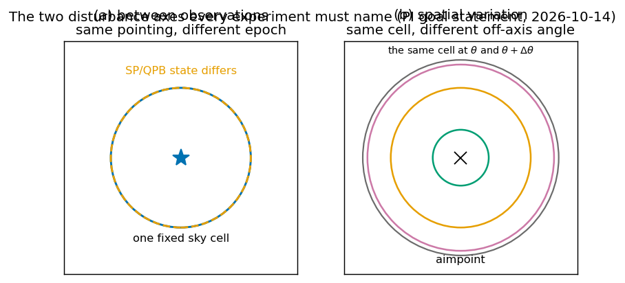
来源：Source: cognition-os/02_CURRENT_QUESTION.md

ARF 与 RMF

ARF and RMF

探测器数出来的不是"每个能量的光子各有多少"，而是"落在每个测量通道里的有多少"。要把两者联系起来，需要两个响应函数：

What the detector counts is not "how many photons at each energy", but "how many landed in each measured channel". Two response functions connect them:

• ARF（auxiliary response file，有效面积文件）。一个随能量变化的数：能量 \(E\) 的光子被这台仪器记录下来的概率（含镜面反射、滤片、坏像素、vignetting）。单位是 \(\mathrm{cm}^2\)。The ARF (auxiliary response file). A number as a function of energy: the probability that a photon of energy \(E\) is recorded by this instrument (mirror reflection, filters, bad pixels, vignetting included). Its unit is \(\mathrm{cm}^2\).
• RMF（response matrix file，响应矩阵）。能量 \(E\) 的光子被记到通道 \(c\) 的概率。它把真实的能量谱"抹开"成测到的谱。The RMF (response matrix file). The probability that a photon of energy \(E\) is recorded in channel \(c\). It smears the true energy spectrum into the measured one.

于是"计数"与"天空"的关系是：观测到的计数 = 真实天空通量 \(\times\) ARF \(\times\) RMF \(\times\) 曝光 \(\times\) 面积。反过去，从计数推天空就要除以后面四项——除错了，天空就错。

So the relation between counts and sky is: observed counts = true sky flux \(\times\) ARF \(\times\) RMF \(\times\) exposure \(\times\) area. Going backwards from counts to sky means dividing by those four factors — divide wrongly and the sky is wrong.

BACKSCAL：谱的面积

BACKSCAL: the area of a spectrum

抽谱时你在源区（source region）放一个圆，在背景区放另一个圆。两个圆的面积不同，所以背景不能直接减，要先按面积归一。BACKSCAL 就是记录这个面积的数：它等于源区里"活"的面积（去掉坏像素、CCD 间隙后的实际可用面积）。

When extracting a spectrum you place a circle on the source region and another on the background region. The two circles have different areas, so the background cannot be subtracted directly — it must first be normalised by area. BACKSCAL is the number that records this area: it equals the "live" area of the source region (the usable area after removing bad pixels and CCD gaps).

面积用角分平方（\(\mathrm{arcmin}^2\)）计。一个半径 \(4'\) 的圆，面积是 \(\pi \times 4^2 = 50.27\ \mathrm{arcmin}^2\)。BACKSCAL 通常比它小，因为 CCD 有间隙、有坏点、有被排除的芯片。

Area is measured in square arcminutes (\(\mathrm{arcmin}^2\)). A circle of radius \(4'\) has area \(\pi \times 4^2 = 50.27\ \mathrm{arcmin}^2\). BACKSCAL is usually smaller, because the CCDs have gaps, bad pixels and excluded chips.

本项目的固定规则：谱的面积永远取 BACKSCAL，不与 cheese.fits 的面积混用（PI 2026-10-13，D013 收尾）。

A standing rule of this project: the spectrum area is always BACKSCAL, never mixed with the area of cheese.fits (PI 2026-10-13, closing D013).

ESAS：减数据流水线

ESAS: the reduction pipeline

ESAS（ESAS = European Space Agency's XMM-Newton Extended Source Analysis Software）是把原始数据变成可拟合产品的一整套 SAS 脚本。它做四件事：选好时间段（GTI）、扣掉点源与展源（掩膜）、估计并扣除 QPB 与 SP、生成谱与图（含 ARF 与 RMF）。本项目检验的引擎叫 esas_data_reduction。

ESAS (the European Space Agency's XMM-Newton Extended Source Analysis Software) is the set of SAS scripts that turns raw data into fittable products. It does four things: select good time intervals (GTIs), mask out point and extended sources, estimate and remove the QPB and SP, and produce spectra and images (with ARF and RMF). The engine this project tests is esas_data_reduction.

三个必须知道的陷阱，都是本项目实测出来的：

Three pitfalls that must be known, all measured by this project:

1. ESAS 的波段文件夹里放的是同一条谱。文件夹名上的 EMINLIST/EMAXLIST 只选图；obj.pi、back.pi、ARF、RMF 都是全能量段的，各波段文件夹之间逐字节相同。波段计数要从谱加 RMF 的 EBOUNDS 取，不能把通道号当成 eV。The ESAS band folders hold the same spectrum. The EMINLIST/EMAXLIST in the folder name selects images only; obj.pi, back.pi, the ARF and the RMF are full-range and byte-identical between band folders. Band counts come from the spectrum with the RMF EBOUNDS, never by treating the channel number as eV.
2. footprint 覆盖一个 CCD 不等于这个 CCD 可用。要看每个观测的异常状态记录（mos*-anom.log）：处于 B 或 I 状态的芯片即使几何上被覆盖也要排除，否则 BACKSCAL 会是 0。A footprint covering a CCD does not make it usable. Read each observation's anomalous-state record (mos*-anom.log): chips in state B or I are excluded even when geometrically covered, or BACKSCAL becomes 0.
3. 产物名里的曝光号每个观测不同。多数是 mos1S001，但 0137551401 是 mos1S002/mos2S003。用通配符找谱（<cam>[SU]NNN-obj.pi，每个文件夹恰好一个），不要硬编码。The exposure id in product names differs per observation. Most are mos1S001, but 0137551401 is mos1S002/mos2S003. Find spectra by glob (<cam>[SU]NNN-obj.pi, exactly one per folder); never hard-code.

来源：Source: cognition-os/PITFALLS.md

Sherpa 拟合与成分

Sherpa fitting and the components

拿到谱之后，要把"天空"从"背景"里拆出来。做法是谱拟合：假设天空由若干已知形状的成分相加而成，每个成分乘一个待定的归一化，然后调整这些归一化（和温度等参数），让模型预测的计数与实测计数最接近。本项目用的拟合器是 Sherpa（CIAO 的一部分），包在 xsherpa 这个工具里。

Once you have a spectrum, you must separate "sky" from "background". The method is spectral fitting: assume the sky is a sum of components with known shapes, each multiplied by a free normalisation, then adjust those normalisations (and temperatures) so the model's predicted counts best match the measured counts. The fitter used here is Sherpa (part of CIAO), wrapped in the xsherpa tool.

天空的成分（本项目关心的）有四个：

The sky components this project cares about are four:

• LHB（local hot bubble，本地热泡）。太阳周围一个低密度热气体的发射，温度约 \(0.1\ \mathrm{keV}\)。LHB (local hot bubble). Emission from low-density hot gas around the Sun, at about \(0.1\ \mathrm{keV}\).
• MW halo（银河系晕）。银河系自己的热晕，温度约 \(0.2\)–\(0.3\ \mathrm{keV}\)。MW halo. Our own Galaxy's hot halo, at about \(0.2\)–\(0.3\ \mathrm{keV}\).
• CXB（cosmic X-ray background，宇宙 X 射线背景）。无数活动星系核的叠加，用幂律描述。点源掩膜去掉了一部分，剩下的叫"未分辨 CXB"。CXB (cosmic X-ray background). The sum of countless active galactic nuclei, described by a power law. The point-source mask removes part of it; what remains is the "unresolved CXB".
• 目标天体的成分。例如 M31 的热星际介质，温度约 \(0.7\ \mathrm{keV}\)。The target's own component. For example M31's hot interstellar medium, at about \(0.7\ \mathrm{keV}\).

背景侧，QPB 用同一区域测得的 -back.pi 乘 BACKSCAL 比例；SP 用一个断折幂律（bknpower，断点能量冻在 \(3.2\ \mathrm{keV}\)）。

On the background side, the QPB is the same region's measured -back.pi scaled by the BACKSCAL ratio; the SP is a broken power law (bknpower, break energy frozen at \(3.2\ \mathrm{keV}\)).

统计：cstat 与 chi2

Statistics: cstat and chi2

X 射线计数服从泊松分布：如果期望计数是 \(\lambda\)，实测到 \(k\) 个的概率是 \(P(k) = \lambda^k e^{-\lambda}/k!\)。计数少的时候，高斯近似不成立，必须用泊松似然。

X-ray counts follow a Poisson distribution: if the expected count is \(\lambda\), the probability of measuring \(k\) is \(P(k) = \lambda^k e^{-\lambda}/k!\). When counts are few, the Gaussian approximation fails and the Poisson likelihood must be used.

两种统计量：

Two statistics:

• chi2（卡方，含 Gehrels 修正）。把每个 bin 的残差平方除以方差再相加：\(\chi^2 = \sum_i (n_i - m_i)^2 / \sigma_i^2\)。它假设计数近似高斯分布。好处是可以直接减背景（减完再算 \(\chi^2\)），坏处是计数少时有偏。 chi2 (chi-square, with the Gehrels correction). Sum the squared residual of each bin divided by its variance: \(\chi^2 = \sum_i (n_i - m_i)^2 / \sigma_i^2\). It assumes the counts are approximately Gaussian. Its advantage is that the background can be subtracted first; its disadvantage is a bias when counts are few.
• cstat（Cash 统计量）。直接最大化泊松似然：\(C = -2 \sum_i [ n_i \ln m_i - m_i - \ln(n_i!) ]\)。它计数少时无偏，但要求模型能预测未减背景的总计数——所以背景必须作为模型的一项，而不是先减掉。 cstat (the Cash statistic). Maximises the Poisson likelihood directly: \(C = -2 \sum_i [ n_i \ln m_i - m_i - \ln(n_i!) ]\). It is unbiased when counts are few, but requires the model to predict the unsubtracted total counts — so the background must be a term of the model, not subtracted first.

本项目实测：在暗天区，\(\chi^2_{\mathrm{gehrels}}\) 比 cstat 高估天空约 \(4\)–\(9\ \%\)（中位），但每次实现的散布有 \(20\)–\(27\ \%\)，所以这 \(4\)–\(9\ \%\) 不是一个可以套用的修正量——它是一个系统误差的下限。结论是：暗天区用 cstat，并且永远把所用估计量与它的误差模型一起报告。

This project measured: in faint fields, \(\chi^2_{\mathrm{gehrels}}\) over-estimates the sky by about \(4\)–\(9\ \%\) (median) relative to cstat, but the per-realisation scatter is \(20\)–\(27\ \%\), so the \(4\)–\(9\ \%\) is not a correction you can apply — it is a floor on the systematic. The conclusion: use cstat in faint fields, and always report which estimator is used together with its error model.

如何给一致性打分

How consistency is scored

一个流水线版本好不好，不看它测得的天空绝对值，而看它在同一天域的多次观测间有多一致。三个量：

How good a pipeline version is, is judged not by the absolute sky it measures but by how consistent it is across observations of the same sky cell. Three quantities:

• 超出散射 \(\tau/\bar{I}\)。对一道题的所有 case，先算加权平均 \(\bar{I}\)（权重 \(w_o = 1/\sigma_o^2\)），再看各 case 相对它的散布。如果散布比统计误差还大，多出来的那部分就是 \(\tau\)（DerSimonian–Laird 估计）。\(\tau/\bar{I}\) 是"系统误差占信号的份额"。 Excess scatter \(\tau/\bar{I}\). For all cases of one problem, first compute the weighted mean \(\bar{I}\) (weights \(w_o = 1/\sigma_o^2\)), then look at the spread of the cases about it. If the spread exceeds the statistical error, the excess is \(\tau\) (DerSimonian–Laird estimate). \(\tau/\bar{I}\) is "the fraction of the signal that is systematic".
• 离轴斜率。把每个 case 的面亮度除以加权平均，对离轴角 \(\theta\) 做加权直线拟合，斜率以"每角分的百分比"报告。 Off-axis slope. Divide each case's surface brightness by the weighted mean, fit a weighted straight line against the off-axis angle \(\theta\), and report the slope in "percent per arcminute".
• 统计噪声 \(\sigma/\bar{I}\)。同样本下的平均统计误差。好的流水线要同时压低 \(\tau/\bar{I}\) 与斜率，而不放大 \(\sigma/\bar{I}\)——否则可以把噪声当一致性。 Statistical noise \(\sigma/\bar{I}\). The mean statistical error for the same sample. A better pipeline must reduce \(\tau/\bar{I}\) and the slope at the same time without increasing \(\sigma/\bar{I}\) — otherwise noise would be mistaken for consistency.

来源：Source: MosaicSelfCal/RESEARCH_PLAN.md